Finding Missing Number(s)

August 28, 2015December 2, 2015 asdyLeave a comment

“A question not simple enough to answer and answer not simple enough to understand”

problem statement-

We have a bag containing numbers 1, 2, 3, …, 100. Each number appears exactly once, so there are 100 numbers. Now few numbers is randomly picked out of the bag. Find the missing numbers.

1. Solution for ‘one’ number missing from the baG

If $S_1$ is the sum of n natural numbers, then $S_1$ can be calculated from the following formula

$S_1 = \dfrac{n(n+1)}{2}$

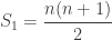
Validity of this formula can be checked with the help of Principle of Mathematical Induction.

$S_1$ is what we expect the bag must be having if all the number were present in the bag. However, one number is missing from the bag and our task is to find that number. We can compute the sum of all numbers currently present in the bag iteratively, say $S_2$ . Difference between $S_1$ and $S_2$ is the number missing from the bag.

pseudocode

1. S = (n*(n+1))/2 
2. numSum = 0 
3. for i = 1 to n 
4.   numSum = numSum + A[i] 
5. return (S-numSum)

Run time complexity of above algorithm in worst-case is $\mathcal{O}(n)$ , which is fairly good. However, one may decide to optimize this algorithm in case of large evil value of n.

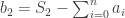
2. SOLUTION FOR ‘Two’ NUMBERs MISSING FROM THE BAG

The above solution works well only if, one number is missing from the list of available numbers. So there may a question that what will be the result produced from the algorithm proposed above when applied in this case? And the answer is sum of two missing numbers. And that is quite obvious to understand from what the above algorithm is trying to calculate. Let us assume that the two missing numbers are $a_1$ and $a_2$ .

$b_1 = a_1+a_2$ $(1)$

$eq(1)$ can be calculated from the algorithm proposed above.

Since there are two unknown variables in $eq(1)$ we need another equation to find missing numbers. Let us say that $b_2$ is the sum of square of two missing numbers.

$b_2 = a_1^2+a_2^2$ $(2)$

And if $S_2$ is the sum of square of n natural numbers then,

$S_2 = \dfrac{n(n+1)(2n+1)}{6}$ $(3)$

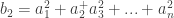
Following to this, we calculate the sum of square of given numbers iteratively in a similar manner we calculated the sum of given numbers in previous case discussed. Difference between $S_2$ and the calculated sum of squares is equivalent to $b_2$ . Thus,

$b_2 = S_2 - \sum_{i = 0}^{n}a_i$ $(4)$

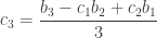
Solving the two equation $(1)$ and $(2)$ for $a_1$ and $a_2$ is our final step towards the solution of the problem. However, this is easier to say than to be done. There do exist different algorithm for solving such equation, you can search for them. Wolfram alpha solves such equation, but what I am not sure about is; their complexity; which will increase as the number of equation increases.

There is a better way of dealing with this problem and I won’t leave that for next time. We will discuss about it in a moment. Till then we can say that solution of the two equations above is the our expected and required answer.

3. SOLUTION FOR ‘k’ NUMBERS MISSING FROM THE BAG

All we now need to do is, generalize our discussion up until now. We need ‘k’ number of equations of missing numbers, which we can solve and find those missing numbers. Again these different equations will be sum of different powers of missing numbers. Since, we need ‘k’ different equation, powers of missing number will range from $i = 1..k$

$b_1 = a_1+a_2+a_3+...+a_n$

$b_2 = a_1^2+a_2^+a_3^2+...+a_n^2$

$b_i = a_1^i+a_2^i+a_3^i+..+a_n^3$

Calculating the value of $b_i$ is entirely similar to what we did in our previous section. Let us assume that we have already computed the the sum of ith powers of n natural number (say $S_i$ ). And what I’m assuming is not hypothetical and would take at most $\mathcal{O}(n)$ . Next thing we need to compute is the sum of ith power of given numbers. Subtracting the two; we get values of $b_i$ where $i = 1..k$ . Good until now.

Now comes the challenging part. At exactly this point I concluded in previous section that the solution of the equations is our required answer. Which is also true in this case. But now, with so many equation in hand entire algorithm might seems an impractical attempt. But, we do have a comparatively easier way of solving these equation. And at this point you will find Newton’s Identities helpful. In case you are not familiar with the concept of Newton’s Identities, please follow the link provided which have a wonderful explanation of Newton’s Identities.

There is something important to explain here. Look at this polynomial equation here –

$f(x) = (x-a_1)(x-a_2)(x-a_3)...(x-a_k)$ $(3)$

$f(x) = x^k-c_1x^k-1+c_2x^k-2+...+c_k$ $(4)$

Coefficients $c_1,c_2,c_3...c_k$ can be calculated with the help of Newton’s Identities as follows

$c_1 = b_1$

$c_2 = \dfrac{b_2-c_1b_1}{-2}$

$c_3 = \dfrac{b_3-c_1b_2+c_2b_1}{3}$

$c_4 = \dfrac{b_4-c_1b_3+c_2b_2-c_3b_1}{-4}$

$c_k = \dfrac{b_k-c_1b_k-1+c_2b_k-2-c_3b_k-3+...+(-1)^{k-1}c_{k-1}b_1}{(-1)^{k-1}k}$

$c_k = \dfrac{b_k-\sum_{i=1}^{k-1}(-1)^{i-1}c_ib_{k-i}}{(-1)^{k-1}k}$

The values computed can be substituted in $eq(4)$ . And our last step is to factorize $eq(4)$ to get equation of the form $eq(3)$ .

Its easier to solve $eq(4)$ than $k$ different equation of different power. If you are looking how, here are few helpful resource links

PSEUDOCODE

1. Calculate sum of ith power of n natural numbers
2. Calculate sum of ith power of given numbers
3. Subtract the result from above two steps to get 
   sum of ith power of missing numbers, say bi. 
   Use generalized formula(from Newton's Identities)
   proposed above to compute coefficients of eq(4).
5. Factor eq(4) after substituting coefficient get polynomial 
   equation of the form eq(3).
6. Roots of eq(4) are the missing numbers.

conclusion

This solution has no practicality, but since we were concerned about time as well as space complexity, we have a good approach to restrict complexity to k not N. Remembering the powers is enough to find the solution of above stated problem. How many powers? Well obviously, k – count of number of elements missing from the bag.

There is another approach to this problem, much more practical than this one but at the cost of complexity. What we can do is sort the given numbers in increasing order ( $\mathcal{O}(nlogn)$ ). And then count along to find those numbers with difference more than one from the previous one [read this]. This is definitely a solution on which everyone can agree. However, the solution presented above becomes more important and and more right when someone explicitly mentions to consider complexities in terms of k not N.

references

Recursive Insertion Sort

July 28, 2015June 1, 2016 asdyLeave a comment

INSERTION-SORT Analogy

“We start with an empty left hand and the cards face down on the table. We then remove one card at a time from the table and insert it into the correct position in the left hand. To find the correct position for a card, we compare it with each of the cards already in the hand, from right to left, as illustrated in figure above. At all times, the cards held in the left hand are sorted, and these cards were originally the top cards of the pile on the table.”

source: Introduction to Algorithm by CLRS

ITERATIVE INSERTION-SORT ALGORITHM

INSERTION-SORT(A) 
1 for j = 2 to length[A] 
2 do key = A[j] 
3   Insert A[j] into the sorted sequence A[1 . . j − 1]. 
4   i = j − 1 
5   while i > 0 and A[i] > key 
6     do A[i + 1] = A[i] 
7     i = i − 1 
8   A[i + 1] = key

Recursive insertion-sort

Insertion sort can be expressed as a recursive procedure as follows. In order to sort A[1 . . n], we recursively sort A[1 . . n−1] and then insert A[n] into the sorted array A[1 . . n − 1].

ALgorithm

INSERT(element, A, n)
1. if n < 1
2.   A[0] = element
3. else if element >= A[n]
4.   A[n+1] = element
5. else
6.   A[n+1] = A[n]
7.   INSERT(element, A, n-1)

RECURSIVE-INSERTION-SORT(A,n)
1. if n < 2
2.   return A
3. else
4.   RECURSIVE-INSERTION-SORT(A,n-1)
5.   INSERT(A[n], A, n-1)

implementation in python

import time

def insert(element, A, n):
    if n &amp;lt; 0:
        A[0] = element
    elif element &amp;gt;= A[n]:
        if n == len(A)-1:
            A.append(element)
        else:
            A[n+1] = element
    else:
        if n == len(A)-1:
            A.append(A[n])
        else:
            A[n+1] = A[n]
            insert(element, A, n-1)

def insertion_sort(A,n):
    if n &amp;lt; 1:
        return A
    else:
        insertion_sort(A,n-1)
        insert(A[n], A, n-1)

A = [5,4,3,2,1]
start_time = time.time()
print(&quot;Unsorted Array: %s&quot; %A)
insertion_sort(A,len(A)-1)
print(&quot;Sorted Array: %s&quot; %A)
print(&quot;--- %s seconds ---&quot; % (time.time() - start_time))

Explanation

Insert is a utility function which recursively adds element in the given array A of size n in order. For example if we use insert to add 1 in an array A = [2] or if we use it to add 2 in an array A = [1]; in both the cases we get A = [1,2]. In the algorithm above we use this function to insert an element A[i] in sorted array A[1..i-1].

Insertion-Sort is a function which takes an array A to be sorted and n (number of element in A). The function recursively call itself to sort sub-array A[1..n-1] and then insert A[n] in A[1..n-1]. This recursive call maintain that insertion of element is performed on a sorted array

DEMONSTRATION OF RECURSIVE CALL

Call INSERTION-SORT with A = [5,4,3,2,1], n = 5
  Call INSERTION-SORT with A = [5,4,3,2], n = 4
    Call INSERTION-SORT with A = [5,4,3], n = 3
      Call INSERTION-SORT with A = [5,4], n = 2
        INSERT 4 in A = [5] and n = 1
        return A = [4,5]
      INSERT 3 IN A = [4,5] and n = 2
      return A = [3,4,5]
    INSERT 2 in A = [3,4,5] and n = 3
    return A = [2,3,4,5]
  INSERT 1 in A = [2,3,4,5] and n = 4
  return A = [1,2,3,4,5]

Analysis

Let $T(n)$ be the running time on a problem of size n.

When $n = 1$ , $T(n) = \Theta (1)$ . However, when $n > 1$ , $T(n)$ is the sum of time taken to sort the array of size n-1 and time taken to insert the last element in the sorted array.

Next question to trigger on is what is the running time of Insert? If we try to analyse we see that the method recursively reduce the array by one to find the right place to fit in the element. For that, in worst case the method will go through each element in the array; which will cost $\Theta (n)$

Thus $T(n) = T(n-1) + \Theta (n)$ for $n > 1$ .

CONCLUSION

After understanding Recursive Insertion-Sort algorithm read the analogy mentioned at the start of this post from the book Introduction to Algorithm. You will find that even in case of Recursive algorithm we maintain that analogy.

There is no extra work to do in case of Recursive Insertion-Sort. Algorithm will first pick up the second element from the array and insert it in the sorted array to its left, currently with only one element. Next it will pick the third element and inserted it in the sorted array to its left which now have 2 element in sorted order. We do this until the last element of array. At last we have a sorted array.

Hello world!

July 28, 2015June 17, 2016 asdyLeave a comment

Those who have their personal WordPress blog up and running might have noticed that I have not changed the default title of the first blog post. Well, that directly links to what I will be posting in this blog. First, lemme introduce myself.

WHO I’M?

I’m Prateek Dwivedi, a student pursuing my Bachelors of Technology in Computer Science Engineering from KCC Institute of Technology and Management, Gr. Noida.

What is this blog about?

This is my personal blog where I will be posting stuff worth sharing on world wide web. Back in the summers of ’15, I realized that there are so many things to share you come across daily. However, I will restrict myself to share stuff I learn in my field of computer science.

Recently I started with Introduction to Algorithm by Thomas H. Cormen, Charles E. Leiserson, Ronald L. Rivest and Clifford Stein. This book is an Ocean of Knowledge. It’s not just about words the authors penned down but it’s also about those exercises and problems the book is full of. Therefore, I might share implementation/solution of few exercises/problems. For more you may like this.

And much more …